

Mapping with UAV systems without the need of Ground Control Points
Mapping with UAV systems without the need of Ground Control Points
The drone and software industry has brought a revolution in the photogrammetry field. Combining the GPS system with the drone technology can provide great results in the creation of aerial photos. The economic advantages of Structure from Motion (SfM) mapping without any ground control points have motivated us to investigate an approach that relies on accurate camera exposure positions instead of Ground Control Points (GCP)
for geo-referencing purposes. This paper describes the possibility to create accurate mapping products, such as Orthophoto and Digital Elevation Model (DEM), by using only the accurate position of the center of aerial photos. The results will indicate that in SfM (Structure from Motion) mapping the use of Camera Exposure positions (CEPs) instead of GCPs does not significantly reduce the accuracy.
Introduction
Small Unmanned Aerial Systems (sUAS) are being used for many different purposes in the daily life. One of the reasons for this trend is the declining costs of these equipments. This has reflected also in the field of photogrammetry where obtaining low cost good quality aerial photography for reconstruction of 3D topography has made it possible to compete with other technologies in the general market. The integration of Structure-from-Motion (SfM) and multi-view stereo (MVS) algorithms into the standard workflow of digital photogrammetry has led to a series of software products that can restitute topography from imagery with an unprecedented level of automation and ease.[i] One of the steps that is very important for creating good geospatial data is the step of Georectification. Georectification means converting the point cloud from an internal, arbitrary coordinate system into a geographical coordinate system. This can be achieved in one of two ways[ii]:
- Direct method, when we know the camera positions and focal lengths.
- Indirect method, when we incorporate a few ground control points (GCPs) with known coordinates. Typically, these would be surveyed using differential GPS.
Using the indirect method with the surveyed GCPs we can achieve great results and have accurate geospatial products. But, the process takes time and you need to use differential method of GPS surveying for the surveyed GCPs. This is reflected to the cost of the geospatial product, which in many cases has prevented us on using the SfM method. The economic advantages of Structure from Motion (SfM) mapping without any ground control points have motivated us to investigate an approach that relies on accurate camera exposure positions instead of Ground Control Points (GCP) for geo-rectification purposes. The main scope of this paper is to show the differences in accuracy between direct method georectification and indirect method. These differences are obtained through an experiment that we have done in Tirana. The idea of the experiment is to create the geospatial product from SfM method with direct georectification and compare the accuracy of this product from the GCPs that are surveyed directly on the field. In this case the GCPs are not used to georeference the 3D model but are used only to check the accuracy of the direct georectification method from camera exposure positions.
[i] Patrice E Carbonneau; James T Dietrich (2016) – Cost‐effective non‐metric photogrammetry from consumer‐grade sUAS: implications for direct georeferencing of structure from motion photogrammetry. Earth Surface Processes and Landforms. 2017, DOI: 10.1002/esp.4012
[ii] Edwin Nissen 2015 – Structure from Motion presentation Colorado School of Mines
Research design and methods
2.1 Study area
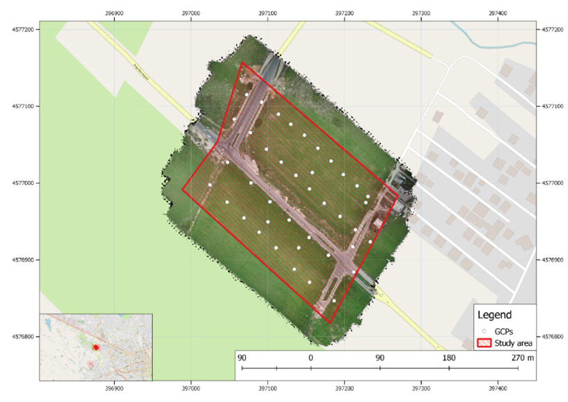
We have performed our experiment in an area near Tirana. Our test area is a 250m x 310m section of a field area with little infrastructure (like roads, etc.) and some buildings. We choose this area because it contains different elements such as infrastructure, fields and several buildings. The area is relatively flat with an elevation between 111m to 121m. For this area, we have surveyed 42 GCPs with two methods:
- Tacheometric method with Trimble S6 Total Station
- Differential GPS method with V-Map System.
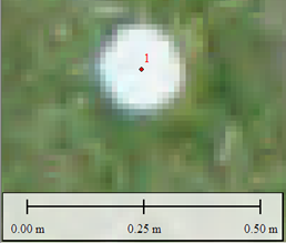
This GCPs are marked on the field to be visible on the aerial photos. Figure 1 shows the study area along with the orthophoto and GCPs.
Field work on the study area
Our field work was done on two days. The first day we started to place the GCPs around the study area and measure them with both surveying methods. The second day we did the UAV aerial survey with V-Map Aerial System.
Surveying of GCPs
After we locate the study area we started to setup a Geodetic network for the surveying of the GCPs. We relied on the ALPOS system for obtaining a base point which was used for both methods of surveying. After the base setup, we started to place on the ground around the field some white plates with 10 cm radius. These plates will be visible on the aerial photos. We spread all the plates around the study area as it is shown in Figure 1. After that we started to do the surveying process with both methods for each of the GCPs. After we did the surveying we decided to go to the office and process the data that we had acquired.
UAV aerial surveying
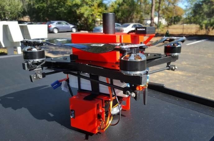
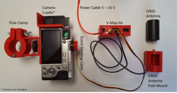
The next day we decided to do the UAV flight with the V-Map Air System Figure 2. Aerial digital photos were acquired using the 20Hz V-Map Air System. Because of weight constraints most small UAVs are equipped with light weight GPS receivers that yield SBAS (WAAS or EGNOS) refined, real time, code based absolute positioning at accuracies typically ranging from one to three meters. While these accuracy levels are sufficient for most navigational purposes, higher levels of accuracy are needed for payloads specifically employed for precision measurements such as 3D modeling of structures by means of photogrammetry or airborne laser scanning. Furthermore, using V-Map to accurately determine camera exposure positions in Structure from Motion (SfM) mapping methods, the need for ground control points can be significantly reduced or, in certain cases, eliminated.[i]
[i] 2016 – V-Map Air System from Micro Aerial Project L.L.C for precise UAV – camera exposure positioning

The standard V-Map system now features the following components and functionalities:
- L1/L2 GPS phase measurements recorded on a micro SD card at 20Hz
- Power input ranging from 5V to 36V
- LED indicator to monitor satellite reception
- LED indicator to monitor proper data storage
- Event marker port
- One PPS outputs
- Removable micro SD card for data retrieval
- Dual frequency helix antenna
The weight of the receiver including external cables and antenna is approximately 120g, which makes it very practical for UAV surveying.
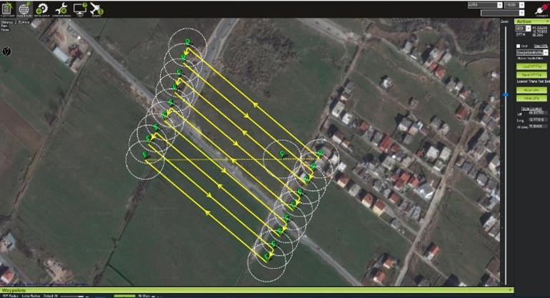
The flight planning was done using Mission Planner Software which is a very useful software that can help you to define the flight itinerary and also can calculate the number of the photos that will be taken. The flight planning is shown in Figure 4.
3D Model Generation
After the field work was finished we started to process the data in the office. By using the V-Map CamPos software we were able to postprocess raw GPS data for camera positions. CamPos has also the option to geotag all the images that were taken with the exact position of the camera exposure. After we finished the process with the CamPos program we had all the necessary data to generate the 3D model by using the AgiSoft Photoscan software. This software uses SfM technique to reconstruct the scene based on a large number of overlapping photos. Photoscan initially detects tens of thousands of features in each image, which are then matched between images. Using the matched features, it is then possible to use an iterative bundle adjustments to estimate the positions of the matched features, positions, orientations and lens distortion parameters of the cameras. This information is used for dense multi-view reconstruction of the scene geometry from the aligned images.[i]
The process of 3D model generation took almost 14 hours to be completed and after that we were possible to get the DSM in 2.5cm pixel resolution Figure 5 along with the orthophoto Figure 6 with the same resolution.
[i] Darren Turner, Arko Lucieer, Steven M. de Jong (2015) – Time Series Analysis on Landslide Dynamics Using an Unmanned Aerial Vehicle (UAV). Remote Sens.2015, 7, 1736-1757; doi;10.3390/rs70201736


Results
In this section, we will present the results of the comparison between GCPs that were measured in two different surveying methods and GCPs positions from the orthophoto Figure 7.
For the comparison of the differences we have used a custom-made program called “V-MAP MakeErrorShapeFile”. This program is used to test the accuracy of our UAV maps by using check points (in addition to Ground Control Points). The check points are pre-marked in the mapping area and surveyed accurately by means of terrestrial methods such as GPS or Total Station.
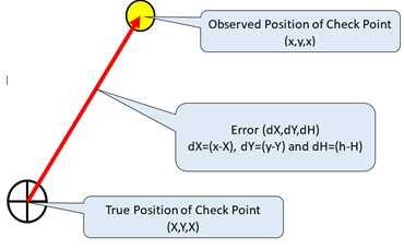
The coordinates (X, Y, H) determined by means of these well-established methods are assumed to be true. To check the accuracy of the UAV-derived Ortho Photo and DSM, we observe the coordinates (x, y, h) of the check points in GIS and then determine the differences dx, dy, dh where dx=x-X, dy=y-Y and dh=h-H. We refer to (dx, dy, dh) as the “error vector”. The coordinate comparison allows us to make the usual statistical analyses such as means, standard deviations and RMSEs. However, without a visualization of the orientation of the error vectors, it is difficult to quickly assess whether there is a bias in the orientation and magnitude of the errors or whether the errors have regional correlation. Since the errors are generally too small to be depicted on a map showing the entire mapping area, it is necessary to show the differences at much larger scale than the mapping scale. A program is thus needed to produce a GIS-compatible file to appropriately display the differences.
A convenient method of 2D visualization is to show the horizontal component of the error vector by means of a magnified arrow pointing from the true position in the direction of the observed position as shown in Figure 8. The vertical component can easily be illustrated by means of either arrow pointing north for positive values and south for negative values or a suitable color based elevation symbology.
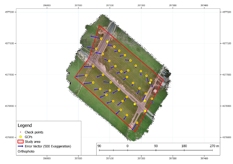
Comparison between Total Station Measurements
Using the program mentioned above we could determine the differences between GCPs measured with Total Station and Check Points from the orthophoto.
After the calculation were concluded through “V-Map MakeErrorShapefile” we can conclude that the Average difference between the Measured GPCs and Check Points from Orthophoto is:
- dx = -0.03143 m
- dy = -0.01569 m
- dh = -0.0763 m
For a detailed statistical information, we are presenting also the Table 1:
Table 1 – Error statistics for difference between GCPs (total Station) and Check Points (Orthophoto)
| dx | dy | dh | ds |
Min | -0.0688 | -0.048 | -0.13124 | 0.015001 |
Max | 0.0125 | 0.017 | -0.04144 | 0.070869 |
Range | 0.0813 | 0.065 | 0.0898 | 0.055868 |
Average | -0.03143 | -0.01569 | -0.07628 | 0.042292 |
Std Dev | 0.020228 | 0.017089 | 0.018105 | 0.012113 |
RMSE | 0.03738 | 0.023197 | 0.078398 |
|
For each Check Point in the orthophoto it is created an error vector which shows the direction of the error. This is illustrated in Figure 9.
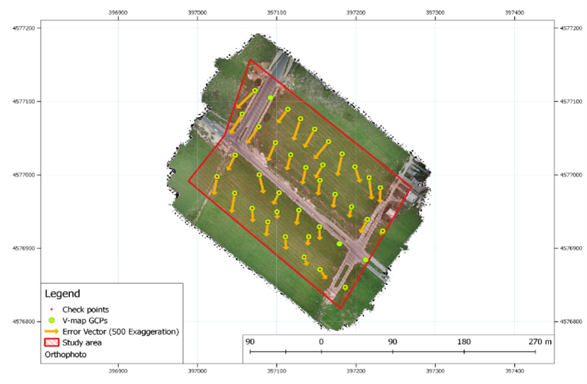
Comparison between V-Map System Measurements
Using the program mentioned above we could determine the differences between GCPs measured with V-map System (Differential GPS) and Check Points from the orthophoto.
After the calculation were concluded through “V-Map MakeErrorShapefile” we can conclude that the Average difference between the Measured GPCs and Check Points from Orthophoto is:
- dx = -0.00929 m
- dy = -0.03983 m
- dh = -0.03505 m
In the second comparison, the differences are smaller than when we compare with the Total Station measurements. The reason for this difference is that the V-Map GPS system that was used for the positions of the camera exposures is the same system that is used for the measurements of the GCPs. This proves that the direct georectification delivers good quality 3D georeferenced model.
For a detailed statistical information, we are presenting also the Table 2:
dx | dy | dh | ds | |
Min | -0.046 | -0.06 | -0.09223 | 0.01 |
Max | 0.016 | -0.01 | 0.017517 | 0.066483 |
Range | 0.062 | 0.05 | 0.109748 | 0.056483 |
Average | -0.00929 | -0.03983 | -0.03505 | 0.042757 |
Std Dev | 0.013987 | 0.012307 | 0.023051 | 0.013836 |
RMSE | 0.016789 | 0.041687 | 0.041951 |
For each Check Point in the orthophoto it is created an error vector which shows the direction of the error. This is illustrated in Figure 10.
Conclusions
The above results indicate that in SfM mapping the use of Camera Exposure Positions (CEPs) instead of GCPs does not significantly reduce the accuracy. With these results, we can conclude that this method can be used for different topographic works like defining the volumes for an excavation site or for surveying purposes. Also with these accuracies the geospatial product that is produced can be very helpful in the cadastral. With the cost of the V-Map Aerial System and the simplicity of which this work is done it can help a lot in creating and updating the cadastral maps.